
H3, or cutting-edge advanced AI methods, build on well-established H1 and H2 AI methods such as image classification and sentence completion. The result is a step change in AI applications, from creating new art and literature to fighting disinformation on social media.
Technological disruption is a daily challenge for businesses, but choosing one technology over another leads to different risks and returns. In order to implement these technologies as part of an enterprise-wide strategy, organizations need to classify these disruptions. This gives them a better idea of what is needed and what is possible.
Horizon 1, or H1 technologies, are well established and used regularly by businesses. H2 and H3 offer potential but aren’t mature enough to be mainstream yet. Although they are still speculative, H2 and H3 technologies could soon disrupt industries and unlock new business models. However, these advances can also create new risks in compliance, safety, and other critical areas.
In this paper, we take a deep dive into advanced game-changing algorithms (blue section of Figure 1) that are now available in the Infosys Enterprise Cognitive platform (iECP). These AI algorithms have been made possible by increased computational power, open datasets, and a mature AI landscape across industries. They follow naturally from advances made in core AI offerings (H1) and experimental AI technologies (H2), which we examine briefly below.
AI core offerings in the H1 category often use mainstream algorithms to understand churn, sentiment analysis, and product or customer recommendations. The algorithms used include random forest, support vector machines (SVM), Naive Bayes, and n-grams.
Figure 1. The AI algorithm horizon

Source: Infosys
The H2 group features new, experimental AI algorithms that are still in a nascent stage of adoption and testing. These will have major benefits and eventually become the mainstream during AI’s second wave.
Convolutional neural networks (CNN) have laid the foundation for computer vision use cases, ranging from object detection to facial recognition to image captioning and segmentation. Long short-term memory (LSTM) and recurrent neural nets (RNN) help significantly improve language translations, sentence formulation, text summarization, and topic extraction.
H3 offerings require more research to understand their nuances, strengths and weaknesses.
Word vector-based models, such as GloVe and Word2Vec, manage large, multi-dimensional text collections and find complex, hidden relationships among topics, entities, and keywords.
H3 technologies are AI’s potential game changers. However, these emerging offerings require more research to understand their nuances and establish their strengths and weaknesses.
Table 1. AI algorithms and use cases
| Horizon 1(mainstream) | Horizon 2(adopt, scale) | Horizon 3(envision, invent, disrupt) | |
|---|---|---|---|
| Algorithms |
|
|
|
| Use Cases |
|
|
|
Explainable AI (XAI)
Neural network algorithms find hidden patterns from data that many other conventional machine learning algorithms, such as SVM, random forest, and Naive Bayes, are unable to establish. Increasingly, organizations are using neural network-based algorithms in hiring, credit lending, and facial recognition. But these systems sometimes produce incorrect and problematic conclusions or decisions. AI results should be justified, explained, and reproduced for consistency and correctness, since the decisions often have profound effects on people’s lives.
Geoffrey Hinton, a University of Toronto researcher often called the godfather of deep learning, explains: “A deep-learning system doesn’t have any explanatory power. The more powerful the deep-learning system becomes the more opaque it can become.”
The answer to this problem is explainable AI (XAI), a way to increase the transparency of black box algorithms and justify how predictions are made. Here are two approaches used to explain AI’s results.
Figure 2. Visual representation of different types of layers
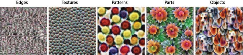
Source: Chris Olah, Google Brain Team
Network dissection helps associate established units with concepts. They learn from labeled concepts during supervised training stages, and discover how and in what magnitude these are influenced by channel activations.
Feature visualization (see Figure 2 above) helps to uncover the layers of a neural network. This was used to understand that lower layers are useful in learning features, such as edges and textures, whereas higher layers are more important for higher order concepts, such as objects.
Frameworks are also improving the explainability of AI models. Two important frameworks are Local Interpretability Model-agnostic Explanations (LIME) and SHAP (SHapley Additive exPlanations).
LIME
LIME treats the model as a black box and tries to create another surrogate non-linear model, where explainability is possible or supported. Different components of an image are evaluated by perturbing the inputs and evaluating its impact on the results, then deciding which parts of the image are most important. Since the original model doesn’t participate directly, it is model independent. However, the surrogate model’s explanations might not be completely generalizable or always one-to-one mappable to the original model.
Figure 3 below shows how a data scientist might use LIME to identify a picture of a tree frog. Create a noisy image by disabling certain features, such as marking portions gray. In this case, calculate the probability that a tree frog is in the image. Using these data points, train a simple linear model, such as logistic regression, to get the results. The superpixels with the highest positive weights become an explanation.
Figure 3. Explaining a prediction with LIME
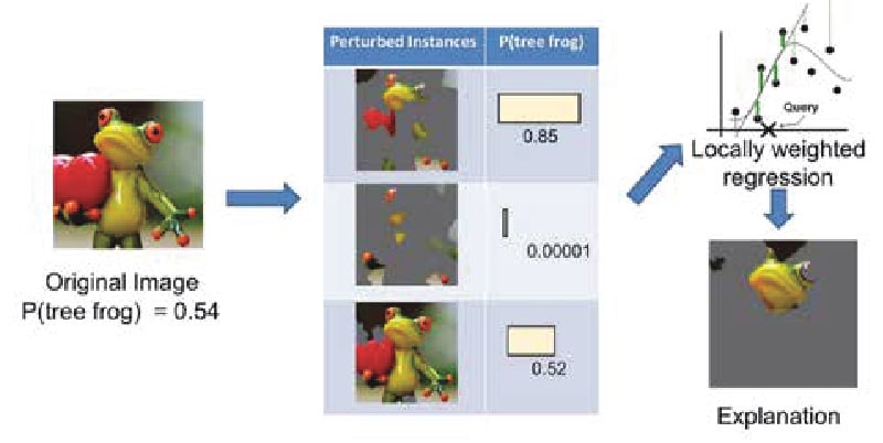
Sources: Marco Tulio Ribeiro, Pixabay
SHAP
SHAP uses a game theory-based approach to predict an outcome. This framework analyzes combinations of features — and their effects on the delta of the results — and then computes the average explainability score for each. For image use cases, SHAP marks the dominant areas by coloring the pixels. SHAP produces relatively accurate results and is more widely used than LIME for explainable AI.
Generative AI
Generative AI offers potential benefits in creative work, such as writing articles, creating new images, improving image or video quality, merging images for artistic creations, creating music, or improving datasets through data generation. Generative AI in the near term will augment many jobs and will potentially replace some as this sub-stream matures.
Generative networks consist of two deep neural networks: generative and discriminative. These work together to provide a high-level simulation of conceptual tasks.
The AI algorithm works by first training the generative model on fresh data, which is then used to generate new data. The new data is then used to fool the discriminative network, which learns by identifying real versus generated data. To get better at speed, the generator — a deconvolutional neural net — trains with an objective function that asks the question: “How well can I fool the discriminator network?” Conversely, the discriminator — a convolutional neural net — is trained on its ability to not get fooled by generated data. Both neural networks learn through something called back propagation.
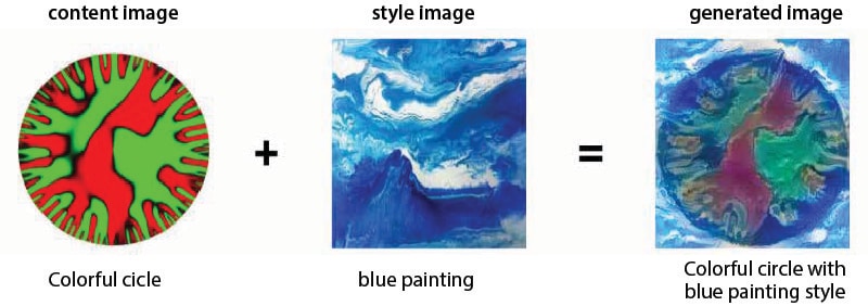
There are different ways of building generative networks, depending on the training objective used. Neural style transfer is a popular generative approach used in image creation. It works by merging two images — a content image (C) and style image (S) — to create a generated image (G) (Figure 4) that is a stylistically perturbed version of the content image.
Other generative algorithms that are currently popular include:
Super-resolution generative adversarial network, or SRGAN — Used to improve image quality.
StackGAN — Used to generate realistic looking photographs from textual descriptions of simple objects, such as birds and flowers.
SketchGAN — A RNN able to construct sketches of common objects. The model is trained on human-drawn images representing many different classes.
Evolutionary generative adversarial networks, or E-GAN — Popular algorithm used by apps such as Snapchat to make younger faces look older, and vice versa.
IcGAN — Used to reconstruct photographs of faces with specific features, including changes in hair color, style, facial expression, and even gender.
Figure 4. Neural style transfer is a generative algorithm combining content and style features
Fine-grained classification
Lower level computer vision algorithms can classify objects (car, table, etc.) with ease. However, H3 algorithms are now making progress by classifying objects using more granular features.
Fine-grained classification is one such algorithm and can be used to recognize car types or species of animals. Clothing firms have monetized this advancement by using granular objects, such as shoes, to help clients find the best style for their wardrobes.
That doesn’t mean it’s easy. Finding discriminative features to train the model is notoriously challenging, as most features are not unique to one object. However, there are a number of new approaches making their way into the mainstream. Those include feature representations that preserve fine-grained information, segmentation approaches that extract purer features, and algorithms that normalize poses of objects to make feature detection easier.
Fine-grained classification often uses an eight-layer CNN, with each layer representing low- to mid- to high-level features. Higher-level features aggregate more complex structural information across larger scales, even capturing and classifying deformed parts of an image. By connecting neural network layers in this way, the model can capture complex relationships between different parts of the image.
Funny enough, bird recognition is a strong use case for the technology. In Figure 5, we see that from the test image, detected key features are first aligned with prototypical models. This information is then fed through the CNN. The features are extracted from multiple layers after which they are concatenated before being fed to a classifier.
Figure 5. Multiple layers of a CNN used to classify a bird through fine-grained classification
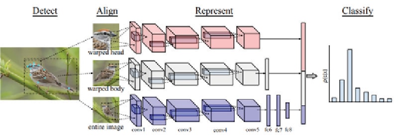
Source: Infosys, Cornell University
Capsule Networks
Convolutional networks are good, though they have their flaws. Because they look at individual features without relating them to a wider consensus of what is actually being described, classification is often incorrect. For instance, if an image of a human face was fed into the CNN, and then features were swapped around (ears for a nose, lips for an eye), the classifier would still understand this to be a regular human face. More discrimination is therefore needed, which is where capsule networks come in. By storing special relationships, they reduce the classification errors and have a greater understanding of what they are actually observing.
Like CNN’s, capsule networks are multi-layered neural networks consisting of several capsules. Each consists of several neurons. In the lower layers, capsules are trained to detect an object, such as triangle or square, within a given region of the image. The output from this layer is a vector with two properties, namely the length and orientation in space. The length attribute is a score for the probability that, say, a triangle or square is present. The orientation is the pose of the object, such as its rotation angle. In the higher layers — known as routing capsules — classification is used to detect and build larger and more complex objects, such as a house or boat (Figure 6).
Figure 6. Capsule network for a house-boat classification example

So, how does the capsule network know how to build the picture of a house in the example above? Routing by agreement is a method by which the capsule network bubbles up higher order features and chooses the right shape via voting.
In the house-boat example, lower levels correspond to the circles-rectangles, and the higher levels corresponds to the house itself. With a circle, the activation vector will be low since it’s not present. The rectangles and triangles will have a high value. Relative positions will bet on the presence of high-level objects. Since they will agree on the presence of a house, the output vector of the house capsule will become large.
Capsule networks work with far less data and fewer parameters than CNN
This then influences the prediction of the rectangle-triangle capsules, which become higher in magnitude. The cycle repeats four to five times, after which the bets on the presence of a house is far higher than that for a boat.
Compared with a CNN, capsule networks need much less data for training and fewer parameters, leading to fewer computations and faster decision making. Further, the capsule networks preserve pose and position and have a much higher accuracy than CNNs, while allowing you to reconstruct the exact image. They are also much better than CNNs at preserving information, especially at the edges of images. With CNNs, edges of rectangles, ovals, and triangles will be preserved using very simplistic kernels, leading to loss of information. This is partly the reason why traditional neural networks don’t handle unseen rotations effectively.
With that in mind, H3 capsule networks are better than traditional CNNS for object detection and image segmentation. Because of their relative immaturity, they are still under heavy research and have not been used on massive computer vision datasets in an enterprise setting.
Meta Learning
Traditional methods of machine learning focus on taking a huge, labeled dataset and then learning to detect y (independent variables such as classifying an image as cat or dog), given a set of x (dependent variables such as images of cats and dogs). An algorithm arrives at various hyperparameters, such as the numbers of layers in the network, number of neurons in each layer, learning rate, weights, bias, dropouts, and activation function (sigmoid, tanh, relu) to activate the neurons. The learning happens through several iterations of forward and backward passes (propagation) by readjusting (learning) the weights based on difference in the loss (actual vs. computed). At the minimal loss, the weights and other network parameters are frozen and considered to be the final model for future predictions. This long, tedious process of repetition for every use case or task is engineering, data, and computing intensive.
Meta learning focuses on how to learn to learn. Human beings have varying styles of learning. Some people learn and memorize with one visual or auditory scan, while others need multiple perspectives to strengthen the neural connections for permanent memory. And many remember by writing or through actual experiences. Meta learning tries to leverage these to build its learning characteristics.
Types of meta learning models
Like human learning techniques, meta learning uses various methods based on patterns of problems, such as boundary space and amount of data, by optimizing the size of the neural network or using a recurrent network approach.
Few-shot — Typically, neural nets require millions of data points to learn. However, few-shot meta learning uses only a small number to build models.
Optimizer — In this method, the emphasis is on optimizing the neural network and its hyperparameters. A great example is models that are focused on improving gradient descent techniques.
Metric-based — The metric space is narrowed to improve the focus of learning in this method. The learning is carried out in this metric space only by leveraging various optimization parameters.
Recurrent model — This is tailored to RNNs, such as LSTM. In this architecture, the meta learning algorithm trains an RNN model to process a dataset sequentially and then process new inputs from the task. In image classification, this might involve passing the set of pairs (image, label) of a dataset sequentially, followed by new examples to be classified. Meta reinforcement learning is an example of this approach.
Figure 7. Transfer learning layers
Source: Infosys, Cornell University
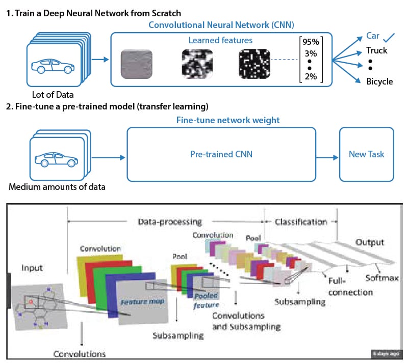
Transfer learning
Humans can learn from both their own experiences and those they have seen, heard, and observed. AI’s transfer learning (TL) discipline is based on similar traits where new models can learn and benefit from existing trained models.
Imagine that a computer vision-based detection model was already able to identify various types of vehicles, such as cars, trucks, and bicycles. However, when an airplane or other new vehicle needs to be detected, researchers would need to retrain the full model or employ transfer learning.
With TL, you can introduce additional layers on top of existing pre-trained layers to start detecting airplanes. Typically, the right weight is reached through many iterations (epochs) of forward and backward propagation. Those take a significant amount of computational power and time. Also vision models need large amounts of image data to be trained.
TL allows data scientists to reuse the existing, pre-trained weights of an existing model. Also, it needs significantly fewer images, just 5% to 10% of those required for training a ground-up model. The pre-trained model has already learned some basics, such as identifying edges, curves, and shapes in the earlier layers. It needs to learn only higher order features that are specific to airplanes. Essentially, TL helps eliminate the need to learn everything from scratch. However, it is important to understand that the TL approach only works now on alike use cases. That means it cannot be used to train facial recognition models.
When using TL, it is important to understand the details of the new use case data since it can implicitly push biases from the underlying data into newer systems. It is recommended that the data and the datasheets of underlying models be studied thoroughly unless the usage is for experimentation purposes.
Although the human brain is used as an example here, it is important to note that people have gone through millennia of evolution and experiences that allow them to learn faster. TL, on the other hand, is just a few decades old and still growing in its use for new vision and text use cases.
Single-shot learning
Humans have the impressive ability to understand new concepts and experiences with just a single example. They can comprehend a new object’s structure and then generate compelling, alternative variations.
Facial recognition systems are good candidates for single-shot learning. The alternative is a system that needs tens of thousands of individual images to train one neural network. That is costly, time consuming, and not always feasible. A single-shot system, using a pre-trained FaceNet model and facial encoding, can be very effective at establishing similarities.
In this approach, a 128-bit encoding of each facial image is generated and compared with other images’ encoding to determine if the person is the same or different. Distance-based algorithms, such as Euclidean distance, can be used to determine if they are within the specified threshold. The model training approach involves creating pairs (anchor, positive) and (anchor, negative). Then the model is trained so that the anchor-positive pair distance difference is smaller and the anchor-negative distance is farther. The anchor is the image of a person for whom the recognition model needs to be trained. Positive is another image of the same person. Negative is a different person’s image.
Figure 8. Single-shot encoding
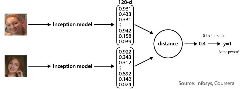
Source: Infosys, Coursera
Deep reinforcement learning
Deep reinforcement learning (DRL) is a specialized machine learning discipline in which an agent learns to behave through rewards or punishments for actions performed (Figure 9). DLR has found significant applications in game design systems, such as chess, AlphaGo, and conventional video games. It is also used for robots, driverless cars, and industrial applications.
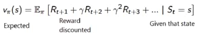
This discipline uses deep learning techniques to bring in human level performance on a given task. The agent can be instructed to maximize short-term or long-term rewards. In reinforcement learning, policy (p) controls what action should be taken. Value function (v) measures the value of being in a particular state. The value function tells us the maximum expected reward the agent will get at each state.
Figure 9. The Q learning notebook

Source: Infosys, Udacity
Three Approaches to Reinforcement Learning
Value-based — The goal is to optimize the value function V. QTable uses any mathematical function to arrive at a state based on actions. The value of each state is the total amount of the reward an agent can expect to accumulate in the future, starting at that state. The agent will use this value function to select which state to choose at each step.
Policy-based — This directly optimizes the policy function (π) without using a value function. The policy is what defines the agent’s behavior at a given time or action = policy(state).
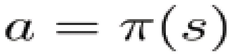
There are two types of policies. The deterministic policy, at a given state, will always return the same action. With a stochastic policy, it outputs a distribution probability over actions.
Value-based and policy-based are more conventional reinforcement learning approaches. They are useful for modeling relatively simple systems.
Model-based — In this approach, a model of the environment’s behavior is created. Then the model is used to arrive at results that maximize short-term or long-term rewards. The model equation can be any equation that is defined based on the environment’s behavior. The model must be sufficiently generalized to counter new situations.
When a model-based approach uses deep neural network algorithms, so the environment’s complexities are well generalized and learned for optimal results, it is called deep reinforcement learning. The challenge with model-based approaches is that each environment needs a dedicated trained model.
AlphaGo was trained using data from several games to beat humans in the game of Go. The training accuracy was just 57%, but it was sufficient to beat people. The training methods involved reinforcement learning and deep learning to build a policy network that tells what moves are promising. And a value network assessed the quality of the board position. Searches for the final move from these networks used the Monte Carlo tree search algorithm. Using supervised learning, a policy network was created to imitate the expert moves.
In 2017, Deep Mind released AlphaGo Zero, which was able to beat AlphaGo without any training from previous game data. The deep network training was done by picking samples from games that AlphaGo and AlphaGo Zero played against themselves. The best moves were selected to train the network and then applied to real games to improve the results iteratively. This is possible because deep reinforcement learning algorithms can store long range tree search results to find the next best move and also perform very large computations.
AutoML
Designing machine learning solutions requires many complex steps and people with a range of skills. They need to collect, understand, cleanse, and normalize the data. Expertise is needed for feature engineering, selecting or designing the algorithm, choosing the model architecture, selecting and tuning the model’s hyperparameters, evaluating the model’s performance, and deploying and monitoring the machine learning system. This requires the expert hands of data scientists.
The complexity of these and other tasks can easily get overwhelming. However, the rapid growth of these applications has created a demand for off-the-shelf machine learning methods that can be used easily and without expert knowledge. The AI research area that encompasses progressive automation of machine learning pipeline tasks is called AutoML or automatic machine learning.
Google CEO Sundar Pichai wrote, “Designing neural nets is extremely time intensive, and requires an expertise that limits its use to a smaller community of scientists and engineers. That’s why we’ve created an approach called AutoML, showing that it’s possible for neural nets to design neural nets.”
Google’s head of AI, Jeff Dean, suggested that 100x computational power could replace the need for machine learning expertise. AutoML vision relies on two core techniques: transfer learning and neural architecture search.
Implementing AutoML
Auto-sklearn automates important tasks in the machine learning pipeline, such as addressing column missing values, encoding categorical values, data scaling and normalization, feature pre-processing, and selection of the right algorithm with hyperparameters. The pipeline supports 15 classification and 14 feature processing algorithms. Selection of the right algorithm can happen based on ensembling techniques and applying meta knowledge gathered from executing similar scenarios (datasets and algorithms).
Figure 10. How AutoML works

Source: AutoML.org
Auto-sklearn is written in python and can be considered as a replacement for scikit-learn classifiers. Here is a sample set of commands:
- import autosklearn.classification
- cls = autosklearn.classification. AutoSklearnClassifier()
- cls.fit(X_train, y_train)
- predictions = cls.predict(X_test, y_test)
Sequential model-based algorithm configuration (SMAC) is a tool for automating certain AutoML steps. SMAC is useful for selection of key features, hyper parameter optimization, and to speed up algorithmic outputs.
Bayesian Optimization Hyperband searches (BOHB) combines Bayesian hyperparameter optimization with bandit methods for faster convergence.
Google and H2O also have their respective AutoML tools which are not covered here but can be explored in specific cases.
AutoML needs significant memory and computational power to execute its alternate algorithms and compute results. Currently, the availability of GPU resources makes it expensive to execute even simple machine learning workloads, such as a CNN algorithm to classify objects. If multiple alternate algorithms were executed, the cost would be exponentially higher.
Adoption of AutoML will depend on two factors: maturity of the AutoML pipeline and how quickly GPU clusters become cheaper. Selling cloud GPU capacity could be one motivation of the cloud-based infrastructure companies that promote AutoML. Also, AutoML will not replace the data scientist’s work but can provide augmentation and speed up certain tasks, such as data standardization, model tuning, and trying multiple algorithms. These are the early days for AutoML, but the technique is a promising option for solving ultracomplex problems.
Neural architecture search
Neural architecture search (NAS) is a component of AutoML and addresses the important step of designing neural network architecture.
Getting neural network architecture right requires quite some work. Neural networks need to be established and organized, the number of filters or channels decided, and other hyperparameters such as filter sizes optimized. This requires several rounds of computation and the work of an expert data scientist. However, since the AlexNet deep neural network architecture won the ImageNet competition in 2012 by a significant margin (using image classification), new architectures have evolved. These include VGG, ResNet, Inception, Xception, InceptionResNe, MobileNet and NASNet. But choosing the right architecture for the right problem is still a niche skill, with each data scientist combing through parameters such as algorithm accuracy, number of parameters, memory, computational footprint, and size of the architecture. Chosen carefully, the right architecture will improve functional efficiency.
NAS speeds up the process by automatically selecting the optimal architecture to solve a given problem.
Figure 11. Neural architecture search is a component of AutoML

Source: what-is-neural-architecture-search
Key Components of NAS
Search space — This provides the search boundary for a specific architecture. Computer vision-based uses, such as scene captioning or product identification, use a definite neural architecture, whereas speech or unstructured text use cases require another. This means that the right architecture must be chosen for the right use. The search space provides a catalogue of best in class architectures for the problem at hand, using domain data and other performance parameters hand crafted by an expert data scientist.
Optimization method — Once the search space is found, the optimization mechanism searches to find the best architecture. Different algorithms are used here, including random sampling or ML evaluation using Bayesian methods. Reinforcement learning can also be used to optimize for the right architecture.
Evaluation method — This step basically evaluates the chosen architecture from the optimization output function. It can be carried out using a full training approach. However, for speed and computational efficiency, partial training can be carried out before applying specialized methods such as early stopping, weights sharing, and network morphism.
NAS has outperformed manual ways of finding the right problem spaces for neural architecture, and shows much promise for the future. However, work is still in progress and NAS is still not ready for production.
Figure 12. NAS determines the search space, optimization method, and evaluation method

Source: https://www.oreilly.com/ideas/what-is-neural-architecture-search
H3: The Infosys way
These ten algorithms are key H3 areas. However, they are certainly not an exhaustive list of the work done in this space. Transfer learning, capsule networks, explainable AI, and generative AI are right at the forefront of AI thinking and look like highly promising areas for industry use cases. At Infosys, we are building early H3 use cases and embedding them into the iECP platform to solve interesting client problems. Figure 13 illuminates a few of these use cases across the ten H3 trends discussed in this paper.
Figure 13. Use cases across H3 that are being developed at Infosys
| Trend | Use cases | |
|---|---|---|
| 1. | Explainable AI (XAI) | Applicable across problem areas where results need to be verified, including tumor detection, mortgage rejection, and candidate selection |
| 2. | Generative AI-Neural style transfer (NST) | Art generation, sketch generation, image or video resolution improvements, data generation-augmentation, music generation |
| 3. | Fine-grained classification | Vehicle classification, type of tumor detection |
| 4. | Capsule networks | Image re-construction, image comparison-matching |
| 5. | Meta learning | Intelligent agents, continuous learning scenarios for document review and corrections |
| 6. | Transfer learning | Identifying a person not wearing a helmet, logo-brand detection in an image, speech model training for various accents and vocabularies |
| 7. | Single-shot learning | Face recognition, face verification |
| 8. | Deep reinforcement learning (RL) | Intelligent agents, robots, driverless cars, traffic light monitoring, continuous learning scenarios for document review and corrections |
| 9. | AutoML | Invoice attribute extraction, document classification, document clustering |
| 10. | Neural architecture search (NAS) | CNN or RNN based use cases such as image classification, object identification, image segmentation, speaker classification |
Source: Infosys Research
References


To maximize the benefits of AI technology, businesses must consider where to use it, and how it can augment or accelerate human processes.
- 16 Jan, 2024
- 15 min read

Ways in which businesses can use AI-driven tools, data, and analytics to increase organic revenue growth profitably.
- 16 Jan, 2024
- 8 min read

Real-time, robust data will provide governments with a soft and directed plan to reopen the economy.
- 08 Jun, 2020
- 14 min read